Program Report: International Finance and Macroeconomics, 2024

Affiliates of the International Finance and Macroeconomics (IFM) Program study financial interactions among nations, including cross-border capital flows, exchange rates, responses to global financial crises, and the transmission of economic shocks. Rather than attempting to summarize the more than 1,000 working papers these researchers have distributed since the last program report in 2015, we focus here on three issues that have attracted substantial research attention from this group: impacts of the COVID-19 pandemic, global supply chain shocks, and the privileged position of the US dollar in global asset markets.

Impact of the COVID-19 Pandemic

The COVID-19 pandemic was a large, global shock with long-lasting economic impact. About a quarter of the IFM working papers submitted since 2016 relate directly to this shock and its aftermath. Figure 1 illustrates the magnitude of the COVID-19 shock around the globe. The impact on the United States was dramatic: a 10 percent decline in GDP between the second quarter of 2019 and the second quarter of 2020. Peru, India, Spain, and the United Kingdom suffered declines in economic activity in excess of 20 percent.¹ Economists deployed a wide range of tools to try to make sense of both the magnitude of the decline in economic activity as well as its transmission through the population and across national borders. One approach, illustrated in research by Zachary Bethune and Anton Korinek; Anand Chopra, Michael Devereux, and Amartya Lahiri; and Alexander Chudik, M. Hashem Pesaran, and Alessandro Rebucci, incorporates the Susceptible, Infected, and Recovered framework of viral transmission into a macroeconomic model that highlights the trade-off between lockdowns to limit contagion and the consequent decrease in income.² Workplace interactions cause the disease to spread, illness reduces productivity and causes workers to retreat from the workplace, and, ultimately, high rates of infection prompt governments to impose policies on social distancing.

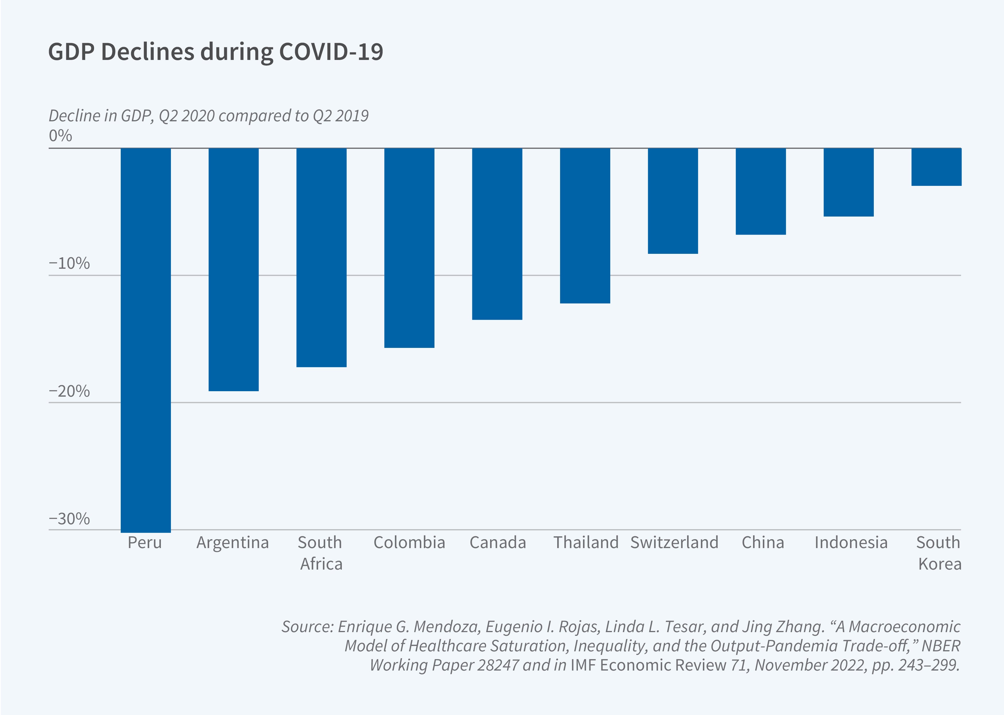
Taking a slightly different perspective, Enrique G. Mendoza, Eugenio I. Rojas, Tesar, and Jing Zhang use international evidence to show that saturation of the healthcare systems — rather than high infection rates — trigger costly economic lockdowns.³ They document that shutdowns happen even when infection rates are relatively low due to bottlenecks in the healthcare sector. In the acute phase of the crisis, lower-income countries were less likely to impose strict lockdowns and therefore experienced larger mortality rates. Cristina Arellano, Yan Bai, and Gabriel P. Mihalache find that countries with less borrowing capacity face tighter fiscal constraints, making lockdowns more costly and constraining policymakers’ ability to impose lockdowns and limit the spread of the disease.⁴ Laura Alfaro, Oscar Becerra, and Marcela Eslava examine the transmission dynamics of COVID-19 in emerging markets, where a greater share of economic activity is conducted by small, informal firms that cannot pivot to working remotely.⁵

At the outbreak of the pandemic, uncertainty over the severity and duration of the crisis triggered a sudden increase in excess demand for liquid assets and a sudden drop in forecasts of future economic activity. Banks and nonbank financial institutions increased their holdings of precautionary cash balances; at the same time, firms drew down their bank lines of credit, generating a spike in risk premia and a fall in equity returns.⁶ Linda S. Goldberg and Fabiola Ravazzolo, and Michael Bordo, document how, in response to this dash for cash, the Fed injected liquidity by providing swap lines and central banks worked in concert to prevent a global financial crisis.⁷ The flight to safety in times of uncertainty underscores the critical role of the dollar during times of volatility, a topic that we will return to below.

Policy during COVID

Provision of liquidity was just the first of many policy measures undertaken to support the fragile global economy. To offset the negative impact of the pandemic, governments provided loans to firms, made transfer payments to households, expanded unemployment coverage, intervened in foreign exchange markets, relaxed macroprudential regulations on financial institutions, and lowered interest rates. Though the set of policy instruments deployed was similar across countries, the precise policy mix varied widely, as pointed out by Joshua Aizenman, Yothin Jinjarak, Hien Nguyen, and Ilan Noy.⁸ Studying a large cross-section of countries, Katharina Bergant and Kristin Forbes find that the choice of policy instrument is strongly influenced by the “policy space” available for that particular tool.⁹ For example, countries with low interest rates entering the pandemic had less capacity to lower rates further; countries with lax financial regulations had less capacity to loosen regulations. Interestingly, a lack of fiscal space did not constrain advanced economies from using fiscal policy despite their entering the pandemic with high levels of sovereign debt.

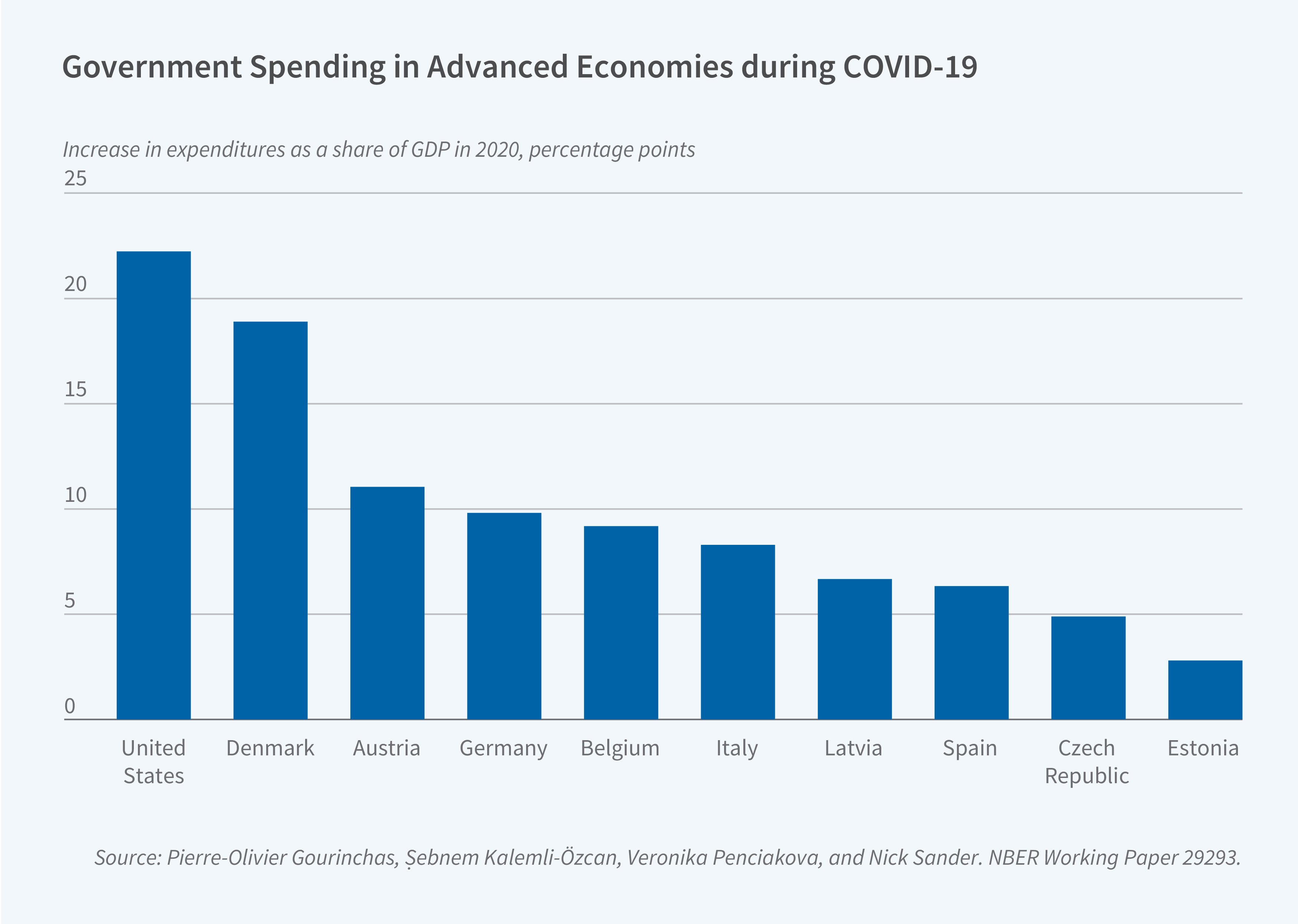
Figure 2, from a study by Pierre-Olivier Gourinchas, Şebnem Kalemli-Özcan, Veronika Penciakova, and Nick Sander, shows the increase in fiscal expenditures as a share of GDP in 2020.¹⁰ The increases in spending were unprecedented for peacetime governments — an average 16.6 percentage point increase in advanced economies. In addition, there were large increases in “below the line” loans and guarantees to households and firms in much of Europe. Fiscal spending was more modest in emerging markets, where it was limited by the degree to which those governments could engage in debt-financed spending.

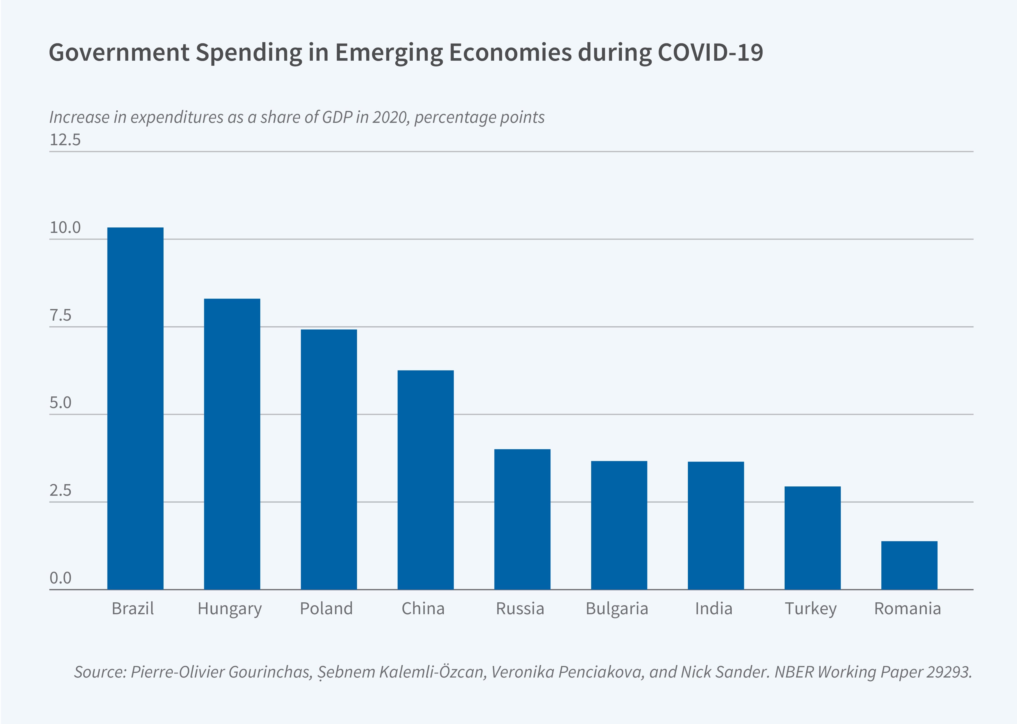
Did this unprecedented level of spending help support struggling firms? Gourinchas et al. drill down to examine the impact of fiscal policy on small and medium-sized enterprises across 27 countries and 50 sectors. Among their many findings, they report that fiscal policy succeeded in preventing widespread failures of small and medium-sized firms, but was less successful in targeting the firms that needed the most help. Fiscal expansion in advanced economies had small or even negative spillovers to emerging markets, and therefore did not make up for the smaller fiscal packages in emerging markets.

Global Supply Chains and Inflation

The pandemic underscored the world’s vulnerability to supply chain disruptions. Tensions between the United States and China prior to the pandemic had already induced many multinationals to reorient their supply chains toward trading partners deemed friendlier to US interests or to on-shore their activities. Lockdowns and plant closures in China during the pandemic put pressure on an already strained global supply network. Bottlenecks in transportation and at ports of entry delayed delivery of final goods as well as intermediate inputs used in manufacturing. These disruptions led some policymakers to question the benefits of trade and to push for further renationalization of supply chains. Barthélémy Bonadio, Zhen Huo, Andrei A. Levchenko, and Nitya Pandalai-Nayar quantify the role of supply chains during COVID using a general equilibrium framework that captures the input-output linkages between industries and across borders.¹¹ They find that about a quarter of the decline in economic activity during COVID can be attributed to global supply chain disruptions. Further, counterfactual exercises suggest that a renationalization of supply chains, reducing reliance on international product flows, would only exacerbate the output decline. Because COVID effects tend to be localized by country and sector, renationalization makes firms more dependent on suppliers that are also experiencing the negative shock.

Negative shocks to supply due to lockdowns and global supply chain bottlenecks coincided with a shift in demand away from services and toward goods. Consumption of goods was further boosted by fiscal transfer payments. An increase in household demand coupled with low interest rates resulted in rising inflation rates around the world. While the initial run-up in inflation could be attributed to negative supply shocks, including disruptions in energy markets due to Russia’s war on Ukraine, the persistence of inflation suggested that relative price increases were passing through to generalized increases in wages and prices. The challenge facing central banks was to see through the supply-side inflation factors and adjust monetary policy to fight demand-driven inflation. In a sample of 10 countries, Galina Hale, John C. Leer, and Fernanda Nechio find that a 10 percent increase in fiscal support directed to households generated a 40 basis point increase in the inflation rate.¹² Focusing specifically on the United States, Julian di Giovanni, Alvaro Silva, Muhammed A. Yildirim, and Kalemli-Özcan conclude that over the 30 months following the COVID outbreak, shocks to aggregate demand accounted for roughly two-thirds of US inflation, and fiscal stimulus contributed half or more of the demand effect.¹³

Exchange Rate Determination

Exchange rate volatility and the fact that this volatility appears disconnected from other macroeconomic variables have challenged international economists since at least the end of the Bretton Woods era. Recent research finds that nominal exchange rates are primarily driven by shocks originating in financial markets, whether due to noise/liquidity traders, preference shocks, convenience yields, or other shifters. This work has revived a focus that had flourished in the 1970s and 1980s on intermediation frictions. Much of the current work is focused on embedding these frictions in open economy general equilibrium frameworks.

Xavier Gabaix and Matteo Maggiori, for example, construct a general equilibrium model that places financiers at the core.¹⁴ These intermediaries are the only conduit for households in different countries to trade intertemporally or share risk. However, they are subject to a constraint on the size of their net exposure to currency movements, requiring a premium to hold large open positions. This mechanism provides a modern take on the classic portfolio balance model developed by Pentti Kouri. Exchange rates in the model are disconnected from macroeconomic fundamentals and are instead driven by financial shocks to relative currency demand.

In a series of papers, Oleg Itskhoki and Dimitry Mukhin study a general equilibrium framework that nests a range of potential shocks, including shocks to wages, time preference, productivity, government spending, markups, the law of one price, the demand for foreign goods, and international asset demand.¹⁵ The last can proxy for preferences for particular assets, noise trading, risk-bearing capacity, expectation errors, or attitudes toward risk. They argue that international asset demand shocks are crucial in generating exchange rate disconnect. They show this analytically for an economy that approaches an autarky limit as well as computationally for a calibrated version of their general equilibrium model. Their study takes this framework to the collapse of Bretton Woods and shows that it is possible to generate a sharp increase in real exchange rate volatility once a currency begins to float. The key insight is that financial intermediaries are unwilling to bear the risk of completely offsetting noise traders when the exchange rate is volatile and that, conversely, under a peg, intermediaries have a more elastic demand for currencies due to the low-risk environment. Thus, a change in exchange rate regime induces a dramatic shift in the relevance of noise traders. The researchers use their framework to argue that financial market shocks take the lead role in generating a host of exchange rate puzzles, with nominal rigidities — the traditional focus of the literature — recast as a supporting player.

Global Safe Asset/Dollar Pricing

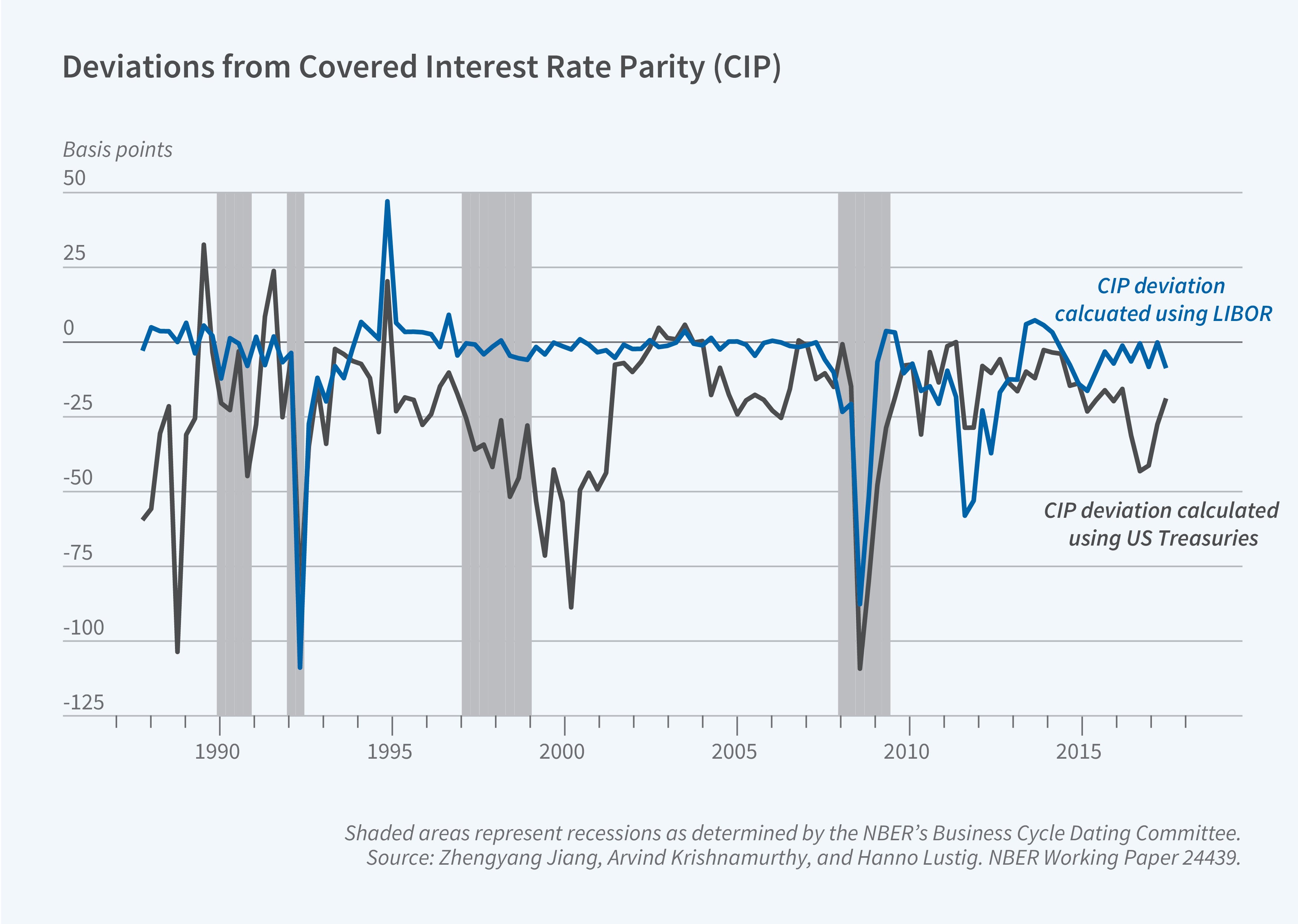
One striking feature about international asset markets is the privileged role of the US dollar. Wenxin Du, Joanne Im, and Jesse Schreger, as well as Zhengyang Jiang, Arvind Krishnamurthy, and Hanno Lustig, show that returns on US Treasuries are consistently below those of similar bonds issued by other G10 economies, even after adjusting for exchange rate risk.¹⁶ In particular, consider the return on US Treasuries minus the yield on a foreign bond plus the difference between the log forward and spot exchange rates in foreign currency per dollar. This is the gap in the covered interest rate parity (CIP) condition for government bonds. If the sign of this expression is negative, then the US bond return is less than a synthetic dollar bond constructed from a foreign bond. Figure 3 plots the time series of the mean and median excess returns on one-year bonds for the US versus nine other developed economies. For comparison, the figure also contains the CIP deviation using the London Interbank Offered Rate (LIBOR), a measure of yields for nongovernment assets. The US Treasury deviation is persistently and significantly negative, with a substantial degree of volatility. Consistent with the important finding of Alexander Tepper, Adrien Verdelhan, and Du, the LIBOR CIP deviation is most prominent after the Global Financial Crisis of 2008.¹⁷ Jiang, Krishnamurthy, and Lustig argue that fluctuations in the implied convenience yield of the dollar are a prime explanatory variable for its exchange rate volatility.

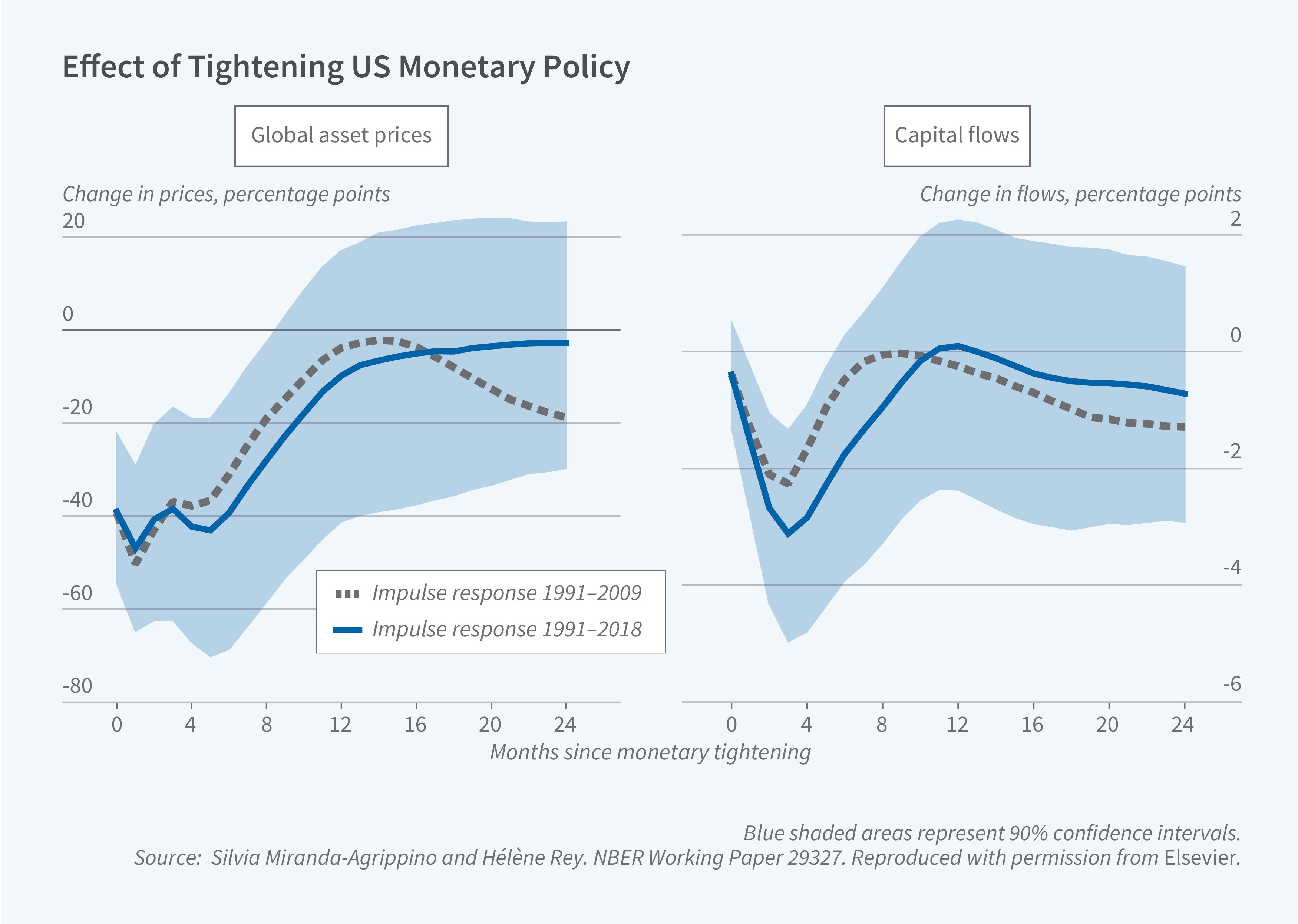
The special role of the dollar contributes to the influence of US monetary policy in the world economy. Silvia Miranda-Agrippino and Hélène Rey document and analyze the fact that capital flows and asset prices around the world co-move strongly with each other.¹⁸ Moreover, a significant driver of these movements is surprises in US monetary policy decisions. Figure 4 shows the impulse responses to a US monetary policy shock for Miranda-Agrippino and Rey’s measure of the global factor in asset prices (left panel) and capital flows (right panel). Surprise US monetary policy tightening generates a global decline in asset prices and a retrenchment in international capital flows.

Kalemli-Özcan shows that US monetary policy shocks affect emerging markets and advanced economies differently.¹⁹ In particular, emerging markets tend to match a US rate increase more than one-for-one, while the pass-through for advanced countries is smaller. Despite the increase in the rate differential between emerging markets and the US, capital tends to flow out of emerging markets. Kalemli-Özcan uses additional measures of risk tolerance to argue that the changing appetite for emerging market risk, and the subsequent increase in the equilibrium risk premium, drives the negative correlation between interest rate differentials and capital flows.